Fundamentals of Modern Statistics Samples and Regression

go back (07.13.05/08.23.2008)

DrTim homepage link

Fundamentals of Modern Statistics Samples and Regression
by Timothy Bilash MD MS OBGYN
July 2005
www.DrTimDelivers.com

based on the book:
FUNDAMENTALS OF MODERN STATISTICAL METHODS
Substantially Improving Power and Accuracy
Rand R. Wilcox (2001)
-----a unique source for understanding the basis of these methods that is well worth reading

Chapter One - Introduction (p1-8)

Inferential Methods
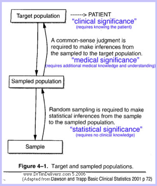
1. Fundamental goal in statistics is to make inferences (assertions) about a large population from a sample subset, especially using small sample size, and in turn whether the population parameters represented by the sample statistics reflect the typical individual. Elements of subjective interpretion are always present in this process.
  
  TDB note: An additional goal in medicine is whether the typical individual represents the patient. Physicians practice clinical medicine (clinical-medical significance), where statistics is just one of the pieces used to diagnose and treat. "Evidence-based medicine", in contrast, presumes that all individuals are represented by the same sample statistic without judgements about individual variation.
2. Implication vs Inference [ANOTE]
  1. distinguish Uni-Directional from Bi-Directional causality.
    1. Uni-Directional Causation is an Implication Forward or Inference Backward , when a risk implies forward or an outcome infers backward (one without requiring the other, not both).
    2. Bi-Directional Causation is an Equality, when a risk implies and an outcome infers from both directions (one requires the other).
  2. These causalities are often confused. The truth of an inverse implication (inference = true) is not equivalent to the forward implication(implication = true). It is more likely true unders some circumstances, but does not have to be, and is a common fatal error of circular logic and decision making.
Normality
1. Jacob Bernouli and Abraham de Moivre first developed approximations to the normal curve 300 years ago (p3-5)
  1. Further development of the normal curve for statistics by Laplace (random sampling) and Gauss (normal curve assumption)
  2. Gauss assumed the mean would be more accurate than the median (1809)
    1. showed by implication that the observation measurements arise from a normal curve if the mean is most accurate
    2. used circular reasoning though: there is no reason to assume that the mean optimally characterizes the observations. it was a convenient assumption that was in vogue at the time, since no way was clear to make progress without the assumption.
    3. Gauss-Markov theorem addresses this
  3. Laplace & vGauss methods were slow to catch on
  4. Karl Pearson dubbed the bell curve "normal" because he believed it was the natural curve.
  5. Practical problems remain for methods which are based on the normal curve assumption
2. Another path to the normal curve is through the least squares principle. (p5-6)
  1. does not provide a satisfactory justification for the normal curve, however
  2. although observations do not always follow a normal curve, from a mathematical point of view it is extrememly convenient
3. "Even under arbitrarily small departures from normality, important discoveries are lost by assuming that observations follow a normal curve." [p1-2]
  1. poorer detection of differences between groups and important associations among variables of interest if not normal
  2. the magnitude of these differences can also be grossly underestimated when using a common strategy based on the normal curve
  3. new inferential methods and fast computers provide insight
Pierre-Simon Laplace method of the Central limit theorem (1811-1814)
1. Prior to 1811, the only available framework for making inferences was the method of inverse probablility (Bayesian method). How and when a Bayesian point of view should be employed is still a controversy.
2. Laplace's method dominates today, and is based on the frequentist point of view using confidence intervals for samples taken from the population (how often a confidence interval around a sample value will contain the true population value, rather than how often an interval around the true population value will contain the sample value).
3. Laplace's method provides reasonably accurate results under random sampling, provided the number of observations is sufficiently large, without the need for an assumption of normality in the population.
4. Laplace method is based on sampling theory. It assumes that the plots of observation means for samples taken from the population have a normal distribution. It is a sampling theory.
5. homogeneity of variance is an additional assumption often made, violation of which causes serious problems

Chapter Two - Summary Statistics (p11-30)

Seek a single value to represent the typical individual from the distribution
1. Area under a probability density function is always one
  1. Laplace distributions example (peaked discontinuous slope at maximum)
  2. many others
2. Probability curves are never exactly symmetric
  1. often a reasonable approximation
  2. asymmetry is often a flag for poor representation by mean
Finite sample breakdown point of sample statistic
1. an outlier is an unusually large or small value for the outcome compared to the mean
2. breakdown point quantifies the effect of outliers on a statistic
3. breakdown point is the proportion of outliers that make the sample statistic arbitrarily large or small (number out of n points, see below)
Mean
1. mean is the simple average of the sample values (ybar)
2. ybar = SUM [y_i]/n
3. mean is highly affected by outliers.
  1. extreme values (Outliers) dominate the mean.
  2. a single outlier can cause the mean to give a highly distorted value for the typical measurement.
  3. arbitrarily small subpopulation can make the mean arbitrarily small or large
  4. has smallest possible breakdown point (1/n). 1 observation or a single point can dominate the mean. it is the most affected by outliers which is not desireable, and why average is easily biased.
4. Weighted Mean
  1. each observation is multipled by a constant and averaged
  2. any weighted mean is also dominated by outliers
  3. sample breakdown point of weighted mean (1/n) is same as for mean (if all weights are different from zero).
Median
1. involves a type of "trimming ", or ignoring contributions of some of the data
2. also orders the observations (which invalidates many statistical tests because violates random sampling)
3. eliminates all highest and lowest values to find the middle one
4. has highest possible breakdown point (1/2). n/2 observations needed to dominate the median, the least affected by outliers (desireable)
Variance (p20-22, 59, 246)
1. A general desire in applied work is measuring the dispersion or spread for a collection of numbers which represent a distribution.
  1. More than 100 measures of dispersion have been proposed
  2. Variance is one measure of the spread about the mean
2. Population Variance = σ ²
  1. average squared deviation from the population mean for single observation (p245)
    1. σ ²= SUM [(population value - population mean)²* (probablity of value)] = expected value of σ ²
    2. s = SQRT [ σ ²] = Population Standard Deviation of an singleobservation from the population mean
  2. convenient when working with the mean
  3. the Population Variance &sigma (for all in the population) is rarely known in practice, but can be estimated by the Sample Variance S of observations in a sample from that population (see below)
3. Sample Variance = S²
  1. the average squared deviation from the sample mean for single observation (p21, see below)
    1. S²= SUM [dev]²/(n-1) = SUM( [sample observations-sample mean]²)/(n-1)
    2. S² = [(y₁-y_bar)² + ... + (y_N-y_bar)²] / (n-1)
    3. Technically distinguished One Sample Mean from Many Sample Variance, calculated as the squared deviation from the Grand Mean. For normal distributions, the Many Sample Variance is the sum of the single sample variances.
    4. n = # in sample, n reduced to (n-1) to adjust for endpoints (independent degrees of freedom)
    5. (y-ybar) = deviation for a single observation in a sample from the sample mean
    6. Sample Variance refers to a Single Sample Variance (SSV). The combined Variance for Many Samples is also called the Sample Variance, and one is an estimate of the other.
  2. Breakdown point of the Sample Variance is the same as for the Sample Mean (1/n)
    1. a single outlier can dominate the value of the Sample Variance S²
    2. low breakdown point of the Sample Variance is especially devastating for determining significance, even when observations are symmetrically distributed around some central value.
4. Variance of the Sample Mean = σ ²/ n
  1. approximates the average squared deviation from the population mean for sample means (p39,71)
  2. variance of the normal curve that approximates the plot of the sample means from the Population
  3. it is centered about the Population Mean, and depends critically on the independence of observations
  4. also calledSquared Standard Error of the Sample Means (SSEM) or Mean Squared Error (MSE)
5. Standard Error of the Sample Mean (SE or SEM) = SQRT [ σ ²/ n]
  1. Square root of the Variance
  2. n = # in sample
  3. measures precision of the sample mean
  4. for normal distributions, also measures accuracy of the sample mean, the closeness of Sample Mean to the Population Mean (makes the sum of the squared Standard Errors equal the square of the summed Standard Errors)
Estimating Population Parameters by Sample Statistics (p59, also see ahead)
1. Population Mean (µ) is estimated by (ybar) the Sample Mean (also by the Grand Mean)
2. Population Variance ( σ² ) is estimated by ( S ² ) the Sample Variance for an observation (single sample)
3. Population Standard Deviation ( σ = SQRT[ σ ² ] ) is estimated by (S = SQRT [S²]), the square root of the sample variance
4. Population Variance of the Sample Mean ( σ ²/ n) is estimated by ( S²/n ), the Single Sample Variance divided by the number in the sample (the single Sample Estimate of the Variance)
5. The terms mean, variance and standard deviation are confusingly used for both population parameters and sample estimates. The distinction between a population parameter (which is a fixed number) and the sample statistic that estimates it (which is a function of the sample) should always be kept in mind. (Mandel p43)
Estimates of statistical closeness of fit (precision) (p22-24)
1. Absolute Value Principle (Boskovich 1700)
  1. calculate the error for value that minimizes the sum of the absolute value errors
  2. uses median value - sample median minimizes the sum of absolute errors
2. Least Squares Principle (Legendre 1806)
  1. calculate the error for the value obtained that minimizes the sum of the squared errors
  2. uses mean values which minimizes the sum of the squared errors
  3. Gauss had used this method earlier but did not publish it until 1809
3. There are are infinitely many other ways to measure closeness in addition to these
  1. essentially arbitrary which measure is used, so some other criteria must be invoked
  2. absolute value to a power
  3. M-estimators of location (Ellis 1844)
  4. >Sample Mean is a special case of M-estimators
  5. many others
Fitting a Straight Line to Data (Principle of Regression p24-28)
1. Background
  1. any two points (x1,y1), (x2,y2) can be used to determine the slope and intercept of a line
    y= intercept + slope*x or (y2-y1)= intercept + slope*(x2-x1)
  2. overdetermined algebraic problem
  3. would get a different line for each pair chosen
  4. N points yields 2N estimates of the slope and intercept
  5. discrepancies are due in part to measurement errors
2. Simple Linear Regression (one predictor, one outcome)(p28)
  2. measure only the linear relationship between the indendent and dependent variable
  3. use the descrepancy between a proposed line (predicted) and the data line (observed)
  4. descrepancy is called a residual
    Residual = r = Y(observed) - Y(expected)
  5. Absolute Residual Method (Roger Boscovich 1700)
    1. minimize the sum of absolute residuals
    2. equivalent to finding the Median
  6. Least Squares Residual Method (Legendre 1809) (p28-30)
    1. unclear if Gauss or Legendre first to use least squares method
    2. minimize the sum of squared residuals, instead of absolute residuals
      1. estimated slope turns out to be a weighted mean of the Y values
      2. equivalently estimated slope is also a weighted mean of all the slopes between all pairs of points
      3. when the slope is zero, the sample mean estimates the intercept
      4. emphasizes values farthest from the mean (a linear method)
    3. find the weighted mean from the infinitely many, which on average is the most accurate
      1. represents the slope and intercept if no measurement errors and infinitely many points
      2. weights are determined by the descrepancy of X-values (predictors) from the mean-X-value
      3. these weights sum to zero, not one
      4. a single unusual point, properly placed, can cause the least square estimate of the slope to be arbitrarily large or small. (breakdown point of 1/N for any weighted mean)
3. Multiple Linear Regression (two or more predictors/risks, one outcome)
  1. predictor independent variables can be numerical or nominal
  2. outcome dependent variables must be numerical only and cannot be nominal
  3. measures only the linear relationship between the independent and dependent variables
  4. there is ambiguity about the term multiple regression. some use the term for multiple outcomes, rather than multiple risks, or even both multiple outcomes and risks
  5. Gauss devised the method of elimination to handle multiple predictors

Chapter Three - Normal Curve and Outlier Detection (p31-48)

Represent the shape of population distribution by fitting a "normal" distribution to it
1. Exponential of [minus the squared deviation from the population mean],
  divided by [the average squared deviation ] (ie, normalized by the variance)
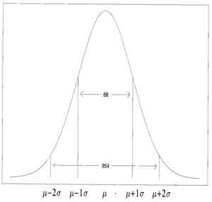
2. 94% of observations are within 2 standard deviations, 68% of observations are within one standard deviation for a normal distribution
3. Mean and Standard Deviation completely represent the distribution if it is normal. Probabilities are determined exactly by the mean and standard deviation when observations follow a normal
Population Distribution versus Distributions of Samples taken from the Population
1. Population Distribution
  1. values for every member of the population
  2. summary parameters for population distribution (population mean and standard deviation as example)
2. Sampling Distribution
  1. repeated, (hopefully) random observations collected in a sample
  2. sample is subset from total population (values for some members of the population)
  3. size (number n) in each sample
  4. "primary" statistics for each sample distribution (sample mean, sample standard deviation and sample variance as examples)
3. Precision
  1. inferences about the sampling distribution (Statistics)
  2. how well sample values represent sample statistic (ie, spread about sample mean)
  3. can estimate precision from the sample data
4. Accuracy
  1. Inferences about the population distribution from the sampling distribution (Statistics + Probablility)
  2. how well sample statistic represents population parameter (spread of single observations or means from sample of observations about the population mean), which depends on
    1. randomness of sampling
    2. size (number) in each sample (n)
  3. inferences using non-random sampling from the population may lead to serious errors.
  4. estimating accuracy from the sample data requires subjective inference in addition to estimating precision
5. Mean, Variance, Standard Deviation for Means for Sample Distributions
  1. Sample Mean is a "primary" statistic from a single Sampling distribution
    1. Sample Variance for observations from a single sample is S²
    2. Sample Standard Deviation for observations from a single sample is S (square root of the Sample Variance)
  2. Mean of Sample Means (Grand Mean) is a "secondary" or summary statistic derived from the distribution of the Sample Means (statistic based on collection of statistics)
  3. Deviations of sample means from the average of sample means form a gaussian (normal) distribution if the samples are random
  4. Standard Error of the Sample Mean (SEM, SE, or Mean Squared Error) is the Standard Deviation for the Means of Samples , relative to a single sample mean (or average of all sample means, the grand mean) used as an approximation to the population mean
  5. Standard Error of the Sample Mean (SE) can be estimated from S as S²/n. This indicates how close (related to percentage of all sample means) any one Sample Mean approximates the average Sample Mean, which both approximate the population mean (statistic + inference)
    1. S² is the Standard Deviation Squared (SD²) for a sample observation (p21).
    2. S²/n is the Standard Error Squared (SE²), the Standard Deviation Squared for a mean of sample observations (approximate, S approximates σ) (p39)
6. Median Absolute Deviation (MAD) Statistic
  1. Want measures of location (representative value) and scale (spread around that value) for a distribution, which are not themselves affected by outliers
  2. Median is one alternative statistic to using mean (middle value)
  3. MAD = median of the [absolute value of the (deviations from the median)] (computed from median of the deviations, see Median)
  4. MAD/.6745 estimates the population standard deviation for a normal probability curve
  5. MAD is less accurate than the sample standard deviation S (computed from mean of the squared deviations) in estimating the population standard deviation σ for a normal distribution
  6. Masking
    1. both the sample mean and sample standard deviation are inflated by outliers
    2. increasing an outlier value also increases the mean and standard deviation for that sample, masking the ability to detect outliers
    3. MAD is much less affected by outliers, so good for detecting outliers (sample breakdown point of 0.5, highest possible)
  7. Outlier Detection using MAD {approximation for |X-Median| = 2.965*MAD }:
    
    |X-Median| > [3*MAD] to determine Outliers
Central Limit Theorem (for samples containing large numbers - due to Laplace p39)
1. Normal Curve
  1. plots of sample means approximately follow a normal curve, provided each mean is based on a reasonably large sample size
  2. this normal curve of sample means would be centered about the population mean.
  3. spread in values obtained from one sampling is called sample variance
  4. the variance of the normal curve that approximates the plot of the means from each sample (variation of the means of samples or SSEM) is estimated by ( σ² / n ) defined using:
    1. population variance ( σ²)
    2. number of observations in a sample ( n ) used to compute the mean
    3. going in inverse order from inference here (use population to estimate the sample)
  5. distinguish SSEM of many samples from the Variance of one sample
  6. non-normality of the parent distribution affects the significance tests for differences of means
  7. there is no theorem to give a precise size for "reasonably large"
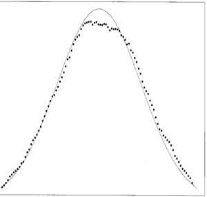
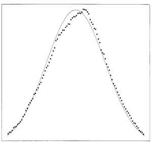
  8. Graphs of (left) Normal Distribution and (right) Medians (used here for illustration, similar to a plot from Means) (dots) of small-sized Samples from Normal Distribution with Expected Normal Distribution from mean and standard deviation (solid), for sample sizes of 20 (fig 3.2 p 34, fig 3.11 p45)
2. [ISLT] curve characteristics relative to the normal curve determine the accuracy of summary statistics
  1. departure from standard bell shape (non-normality, small effect on mean )
    1. if deviations of dependent values (Y's)
  2. skew from symmetry ( bias, large effect on mean)
    1. if asymmetry about the mean, one tail is higher than the other at the same distance from the mean
  3. tails at extreme values ( falloff, large effect on mean and variance)
    1. if convergence slower than normal distribution
  4. summary statistics from non-normal distributions depend both on values in the distribution plus the rate of change in values (ie, second or higher derivatives, or amount of skew compared to normal curve)
3. Uniform distribution example (p40)
  1. constant value from 0 to 1 (all values equally likey, between 0 and 1, step function)
  2. population mean for this curve is 0.5
  3. population variance is 1/12
  4. light tailed and symmetric
  5. central limit theorem predicts that the plot of random small-sample means is approximately normal, centered around 0.5 mean, with variance 1/12N.
  6. plot of only twenty means of samples gives reasonably good results (p40 example).
    1. multiple random sample of twenty values used to predict mean
    2. distribution of these small sample means skewed to slightly higher value
  7. Graphs of (left) Uniform Distribution and (right) Means (dots)of Small-sized Samples from Uniform Distribution with Expected Normal Distribution from mean and standard deviation (solid) (fig 3.5 p40, fig 3.6 p 41)
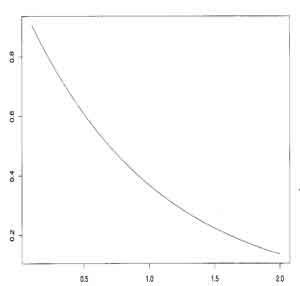
4. Exponential distribution example (p40)
  1. exp(-x) or exp(x)
  2. population mean is 1
  3. population variance is 1/n
  4. light tailed and asymmetric (small samples approximate the normal curve well)
  5. plot of means from samples of only 20 gives reasonably good results assuming the central limit theorem (random small samples of means approximates a normal curve)
  6. plot of means of small sample (n=20) is skewed to slightly lower values for exp(|-x|) compared to large sample means (follows normal curve)
    1. [ISLT] means of small samples from exp(|x|) distribution will be skewed to higher values
      1. exp(-|x|) skewed to smaller values, more so than for a uniform distribution (see p38-40)
    2. Confidence Intervals (CI) of small samples from exp(|x|) are decreased
      1. Confidence Intervals (CI) of small samples from exp(-|x|) are increased
  7. Graphs of (left) Exponential Distribution and (right) Means (dots) of Small-sized Samples from Exponential Distribution with (left) Expected Normal Distribution from mean and standard deviation [solid] (fig 3.7 p41, fig 3.8 p42)
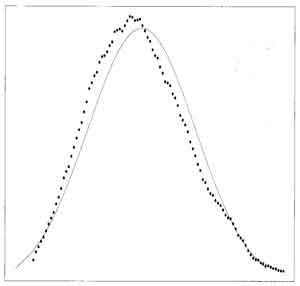
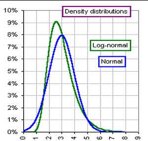
5. Lognormal Distribution Example (p76)
  1. light tailed and highly asymmetric
  2. mean and median are not too far apart since light-tailed, but begins to have problems, especially with Variance estimates. see heavy-tailed "logheavy" below. T-distribution from lognormal begins to have problems because of this.
  3. Graphs of (left) Lognormal Distribution and (right) Means of Small-sized Samples from Lognormal Distribution (green) with Expected Normal Distribution from mean and standard deviation (blue) [from http://www.gummy-stuff.org/normal_log-normal.htm]
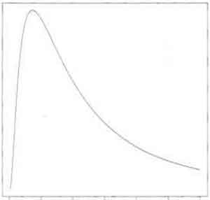
6. "Logheavy" distribution example (p42)
  1. mean and median are very different (contrast with uniform and exponential, where mean and median are close)
    1. heavy tailed and highly asymmetric
    2. outliers more common
    3. mean not near the median
  2. distribution of sample means is poorly approximated by the mean and standard deviation of the sample means (normal approximation) for the "Logheavy" distribution
    1. requires larger numbers for representation of central limit theorem normal approximation, approaching the population mean as the sample size increases.
    2. [ISLT] Accuracy of small samples for "logheavy" distribution
      1. skewing (assymetry relative to central tendancy), departure from linearity, and fall off towards infinity all require larger numbers for normal approximation to be accurate (p44)
      2. high curvature decreases accuracy
      3. slower fall off towards infinity compared to normal distribution (outliers) decreases accuracy
      4. median is different from mean
  3. however, sample median still estimates the population median, even for skewed distributions
    1. small sample mean does not estimate the sample mean for skewed distributions since the mean and median are far apart (population mean far from most of the observations)
    2. faster drop and higher peaked below mean, compensated by slower drop and lower peak above the mean (see fig 3.10)
    3. contrast to lognormal distribution (light tailed)
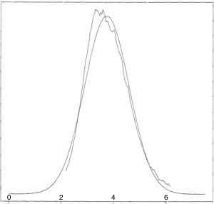
  4. Graphs of (left) "Logheavy Distribution and (right) Means of Small-sized Samples from "Logheavy" Distribution (rippled) with Expected Normal Distribution from mean and standard deviation (solid) (fig 3.9, fig 3.10 p43)
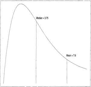
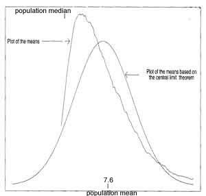
  5. ***"Logheavy" Distribution is much better approximated if use the Medians of Small-sized Samples to approximate population median instead of the Means to approximate population mean (see graph next and p46)
Problems with Samples from Non-Normal Distributions: the Mean and the Median
1. Tails (Light, Heavy)
  1. Tails are how quickly the probablity curve drops off from the mean value towards infinite predictor (X)
  2. Uniform and Exponential distributions are light tailed (drop off quickly towards infinity compared to normal curve, outliers tend to be rare). However the Uniform Distribution is symmetric and Exponential Distribution is asymmetric.
  3. Logheavy distribution is heavy tailed and asymmetric (drops off slowly towards infinity relative to the mean, outliers are common)
2. [ANOTE]
  
  I create terms for the distribution characteristic of "monotonicity" (no change in sign of slope over distribution or wiggles in the distribution curve) and "logheavy" distribution, to be considered with the properties of symmetry (reflection about the mean) and tails (falloff to large/small values) of a distribution
  1. Uniform distribution is ............. light-tailed, symmetric, monotonic (Fig 3.5 p40)
  2. Normal distribution is .............. light-tailed, symmetric, non-monotonic (Fig 3.2 p34)
  3. Exponential distribution is ..... light-tailed, asymmetric, monotonic (Fig 3.7 p41)
  4. Lognormal distribution is ........ light-tailed, asymmetric, non-monotonic (Fig 5.3 p 76)
  5. "Logheavy" distribution is ...heavy-tailed, asymmetric, non-monotonic (Fig 3.9 p43)
  6. these greatly influence statistical behavior and accuracy (if more heavy-tailed, more asymmetric, and less monotonic, then less accurate). light-tails and symmetry are likely to give mean and variance approximations closer to the normal curve. a curve that approximates the normal as the relationship of outcome to predictor values would be called "normotonic".
  7. [ISLT] the combination of these three characterstics tails, symmetry and tonicity relative to the normal distribution curve determine the statistical precision and accuracy. Asymmetric, non-monotonic distributions appear to have unreliable means and/or variances for small samples.
3. Accuracy of sample mean and median (how close statistic is to parameter p44-45, fig 5.5 and fig 5.6 p79-81)
  1. for symmetric probability curves (such as normal)
    1. medians and means of small samples center around the mean/median of a symmetric population (since population mean and median are identical)
    2. normal curve is symmetric about the mean
  2. for asymmetric probability curves
    1. mean
      1. means of small samples are closer to the population median, but slowly converge to an asymmetric population mean as sample size increases, requiring larger sample size to estimate the population mean (p42)
      2. larger samples are needed using means than using medians
      3. this is due to the outliers (one outlier can completely dominate the mean)
    2. median
      1. medians of small samples center around the asymmetric population median
      2. sample median is separated from the asymmetric population mean (in general sample median is not equal to the population mean. see "logheavy" distribution example)
    3. sample medians are a better approximation for the asymmetric population median, than sample means are for the asymmetric population mean with small samples.
  3. for light tailed probability curves
    1. symmetric light-tailed curve- plots of sample means are approximately normal even when based on only 20 values in a sample (p42)
      1. sample mean is close to the median and a good approximation to the population values for symmetric light tailed curves
    2. asymmetric light-tailed- curve can have poor probability coverage for the confidence interval, poor control over the probability of a type I error, and a biased Student's T
  4. for heavy tailed probability curves
    1. symmetric
      1. [ISLT] sample mean is close to median and a good approximation to the population values, however the estimate of the population variance will be inaccurate for heavy-tailed symmetric curves
    2. asymmetric
      1. sample medians provide a better approximation for the population median, than do sample means for the population mean for heavy-tailed symmetric curves
    3. plots of sample means converge much more slowly to the mean for heavy- than light- tailed asymmetric distributions (p45)

Chapter Four - Accuracy and Inference (p49-66)

Errors are always introduced when use a sample statistic (eg, mean for some individuals from the population) to estimate a population parameter (mean for all individuals in the population)
1. can calculate the mean squared error of the sample means (average squared difference)
  1. average or mean of the squared [differences between the infinitely many means of samples (sample means) and the population mean]
  2. called the "expected squared difference" (expected denotes average)
  3. want the mean squared error to be as small as possible
  4. if the mean squared error for the sample mean is small, it does not imply that the standard deviation for a single observation will also be small.
  5. variance of the means of samples is called the squared standard error of the sample mean.
  6. Gauss and Laplace made early contributions for estimating the errors
2. distinguish the sample mean deviation relative to the mean of sample means vs relative to the mean of the population
  1. sample deviations vs population deviations
  2. sometimes these are the same depending on the distributions, and often used interchangeably:
    standard deviation of the mean for a sample
    standard error of the sample mean (standard deviation of the mean of all the sample means)
    standard deviation of the mean for a population
Weighted Means
1. LARGE SIZE, Random Samples (Laplace - Central Limit Theorem)
  1. under general conditions, the central limit theorem applies to a wide range of weighted means
  2. as the number of observations increases, and if repeated the experiment billions of times, would get fairly good agreement between the plot of weighted means and normal curve (can use the mean and standard deviation to estimate the curve)
  3. under random sampling and large numbers, most accurate estimate of the population mean is the usual weighted sample mean. each observation gets the same weight (1/N), based on the average square distance from the population mean.
  4. Assumptions
    1. assumes random sampling
    2. assumes sample sizes are large enough that the plot of means of the samples would follow a normal curve
      1. does not assume that the samples were from a normal population curve
      2. does not assume symmetry in the population curve
2. SMALL or LARGE SIZE, Random Samples (Gauss - General Sample Size)
  1. derived similar results under weaker conditions than Laplace, without resorting to the central value theorem requiring large samples
  2. under random sampling the optimal weighted mean for estimating the population mean is the usual sample mean (as for Laplace formulation). of all the linear combinations of the observations ( weighted means ) we might consider, the sample mean is most accurate under relatively unrestricted conditions that allow the probability curve to be non-normal, regardless of sample size.
  3. Assumptions
    1. random sampling only
      1. does not assume large numbers in sample
      2. does not assume samples were from a normal population curve
      3. does not assume symmetry
    2. used the rule of expected values
  4. there are problems with this approach for some distributions
Median and other Classes of estimators
1. These summary statistics are outside the class of weighted means
2. Sample Median is sometimes more accurate than the sample mean
  1. requires putting observations in ascending order, as well as weighting the observations
Median vs Mean
1. if probability curve is symmetric with random sampling, can find a more accurate estimate of the population mean than the sample mean by looking outside the class of weighted means
  1. Mean
    1. sample mean is based on all the values
    2. nothing beats the mean under normality
    3. tails of the plotted sample means are closer to the central value than the median, so the sample mean is more accurate representation of the population mean
    4. [ANOTE] good for normal/symmetric distributions, otherwise unreliable statistic
  2. Median
    1. not a weighted mean
    2. can be slightly more or greatly more accurate in certain situations
    3. sample median is based on the two middle values , with the rest of the values having zero weight
    4. median is a better estimate of the population mean for Laplace distributions (sharply peaked)
    5. (better for non-normal, symmetric distibutions)
Regression Curve Fitting (Gauss-Markov Theorem) (p55)
1. Simple regression (one predictor variable X, one outcome variable Y)
2. least squares estimator of the slope/intercept of a regression line is the optimal among a class of weighted means
3. does not rule out other measures of central tendancy
4. "homoscedastic" refers to a constant variance (i recommend the term convaried )
  1. population standard deviation (spread in outcome Y) is constant, independent of predictor variable risk X
  2. Gauss showed that if variance is constant, then the Least Squares estimator of the slope and intercept is optimal among all the weighted means that minimize the expected squared error (expected denotes average)
5. "heteroscedastic" refers to a non-constant variance (i recommend the term non-convaried )
  1. population standard deviation or variation in Y values changes with predictor X
  2. Gauss showed that if the variance of the Y values corresponding to any X were know, then optimal weights for estimating the slope could be determined, and derived this result for multiple predictors as well
6. many analysts used the unweighted least squares estimator, assuming a constant variance for the population. however, in some situations, using optimal weighting can result in an estimate that is hundreds, even thousands of times more accurate than the unweighted
Estimating unknown population parameters (making the chain of inference)
1. Each individual is a member of progressively larger (more inclusive) groups
  1. individual sample contains a subset of individuals in the population
    1. sample of individuals drawn at random creates a kind of envelope or shape for the distribution which groups them together (sample curve)
    2. one individual can belong to many different sample groups of the population distribution (different sample curves drawn from the population curve)
  2. individual in the population is a member of the population as well as a member of sample groups
    1. Progression for inference: individual, sample, finite group of samples, infinite group of samples, population
2. An extended chain of inferences is required for validity: individual to sample to finite number of samples to infinite number of samples to population distribution to individual in the population distribution (or mean of sample to mean of finite samples to mean of infinite samples to mean of population distribution to individual in the population distribution)
  1. Parameter reflects some characteristic of a population of subjects
  2. Statistic reflects some characteristic of a sample from that population (primary, or summay secondary)
  3. want to approximate the probability that the population parameter (and thus individual) is reflected by sample statistic. a summary statistic from the sample is used to estimate the corresponding population summary parameter
  4. When use a sample of individuals from the population to estimate the population parameter (for all individuals), always make an error
  5. large number n in each sample requires the central limit theorem (number of samples N )
    1. P_s = sample estimate of a population parameter
    2. SE(P_s) is the standard error of P_s (for number n in each sample) = σ/SQRT (N) ~ S/ SQRT (n). Contrast the sample error of the mean from a single sample versus standard error of the mean for limit of infinite number of samples
    3. CI(P_s, 95%) = CI(P_s, 95% Confidence Interval) = [P_s-1.96*SE(P_s)] to [P_s+1.96*SE(P_s)] which has an approximate 95% probability of containing the unknown population parameter
Estimating the Population Mean (p58)
1. Laplace General method
  1. requires random sampling, which means that all observations in a sample are independent of risks and outcomes
  2. plot of infinitely many sample means assumed to follow a normal curve. this is reasonable for:
    1. large numbers in each sample (use central limit theorem)
    2. normal distribution in population
  3. find an expression for the variance of infinitely many sample means
  4. make a chain of inferences:
    1. find mean of one sample
    2. estimates the mean of many samples
    3. estimates the mean of infinite number of samples
    4. estimates the population mean
2. Standard Deviation ***
  1. confusing terminology (implied by the context)
    1. sample mean refers to the average from one sample , but also used for the average of the means from many (average from single sample vs average from multiple samples)
    2. SD (Standard Deviation) can refer to spread in any collection of individual observations, for a sample, for a population it represents, and also within any grouping
  2. standard deviation for a sample of individuals from the population (S using the sample mean)
    1. approximates the standard deviation of sample means from the grand mean
    2. approximates the population standard deviation σ
Confidence Interval (Laplace 1814 p58)
1. Confidence Interval for a Population Parameter P_s
  1. CI(P_s, 95%) = [P_s-1.96*SE(P_s) to P_s+1.96*SE(P_s)]
  2. P_s = sample estimate of a population parameter
  3. N = number in each sample
  4. SE(P_s) is the standard error of P_s
  5. has an approximate 95% probability of containing the unknown population parameter
  6. this method assumes homoscedasticity. if there is heteroscedasticity , the confidence interval can be extremely inaccurate , even under normality.
2. Confidence Interval for the population mean (µ) (p60)
  1. assumes normal distribution in population and large numbers N in each sample
    1. population mean = ( µ)
    2. population variance = (σ ²)
    3. sample mean variance = ( σ ² / N ) is the squared deviations from µ summed
    4. assumes sample variance ( S ) approximates the population variance ( large numbers in samples, invoke central limit theorem)
  2. CI(µ, 95% population mean)
    1. the interval of +/-1.96 * [SE] = +/-1.96 * [ σ/ SQRT(N) ], has a 95% probability of containing the unknown population mean.
    2. This is an important point, for the confidence interval limits concern only the means of populations from which the samples are taken. The confidence limits are not bounds on a proportion of individuals from the population, and the projection to any individual requires inferences and judgements beyond the statistical analysis. In essence the population distribution must be known to do this.
    3. for large enough samples, the sample approximation +/-1.96 * [S/SQRT(N)] has an approximate 95% probability of containing the unknown population mean
    4. 95% confidence interval (CI) is used routinely for convenience. could be any other percentage also.
    5. Laplace routinely used 3 rather than 1.96
3. Confidence Interval (CI) for the slope of a regression line (Laplace p62-67)
  1. Linear Regression is a Weighted Mean (p46)
    1. repeat an experiment infinitely many times with N sampling points in each experiment
    2. Least Squares estimate of the slope of a regression line to the experimental (Y) results can be viewed as the weighted mean of the outcome (Y) values . (see p28-30)
      [ANOTE]
      1) average of all values vs average of means of all samples of values is the same because linear (a+b)+c = a+b+c , if samples are random and numerous
      2) normal distribution also makes the errors linear
    3. Laplace made a convenient assumption and hoped that it yielded reasonably accurate results
      1. assume large numbers in each sample N (central limit theorem)
      2. assume constant variance (homogenous or homoscedasticity, an important assumption
      3. if a reasonably large number of pairs of observations is used (Laplace), then get a good approximation of the plotted slopes under fairly general conditions
  2. [ANOTE] an experiment implies either a controlled selection or random selection from all the possible selections, with identification and control of all variables that may affect the result (are causative), for each observation, or group of observations, or some used function of the observations. defined selections gives results for a defined subgroup, random selections give results for average of random subgroup. these may or may not be equivalent.
  3. [ISLT] its not the parent distribution, but the distribution of errors (for the mean) and square of errors (for the variance) that has to be linear and homoscedastic
METHOD for Least Squares (p55-62)
1. DEFINITIONS for Least Squares
  1. y=b+ax (theoretical regression line for the population we are trying to estimate)
    1. b is the slope of the regression line for infinite number of points
    2. a is the intercept of the regression line for infinite number of points
  2. n is the number of data points
  3. S_y² = sample variance of all the n number of sample y_i values from the sample mean
  4. y_i =b_i +a_i x_i (line fit for the ith sample data point, i=1 to n)
    1. (x_i ,y_i) is the ith data point
    2. x _i is the mean predictor value for the ith group
    3. y_i is the mean outcome value for the ith group
  5. y=d+cx (arrived at regression line from that sample)
    1. d is the least squares regression estimate of the intercept b for the n data points
    2. c is the least squares regression estimate of the slope a for the n data points
2. ASSUMPTIONS for Least Squares
  1. assume independence of outcome and predictor
  2. constant variance in the population (homoscedasticity)
  3. determine that data does not contradict this assumption
  4. estimate this asssumed common variance (per Gauss suggestion)
  5. this assumption sometimes masks an association detectable by a method that permits heteroscedasticity
3. RECIPE for Variance of the slope = σ_c ² for outcome results Y from Least Squares (p64)
  1. Var(Y) = S_y² estimates the assumed common Variance of each group
    1. compute the Least Squares estimate of the slope (a) and intercept (b) for the n points. compute corresponding n residuals of the computed line from the data curve r_n.
    2. square each n residuals
    3. sum the n results
    4. divide by the number of data pairs of observations minus two (n-2)
4. Result For SLOPE VARIANCE for Least Squares (case of slope = c )
  1. Var(c) = σ_c ² = squared standard error of the least squares estimate of the slope c (p64)
    1. Var(c) = S_y² / [(n-1)*S_x²] = ("squared standard error of the least squares estimate of the slope")
    2. σ_c = SQRT [Var(c)] = S_y / ( SQRT [(n-1)*S_x² ]) = ("standard error of the slope")
    3. [ANOTE] squared error is linear for a normal curve

Chapter Five - Small Sample Size (p67-91)

these methods were developed over the last forty years
1. originally thought that standard methods of inference were insensitve to violations of assumptions
2. it is more more accurate to say that these methods perform reasonably well in terms of Type I errors, or false positive findings of statistical significance, when performing regression
  1. when groups have identical probability curves (shapes)
  2. when predictor variables are independent
3. that is, can detect if two distribution curves are not identical, but dont know if it is because of a difference in means, difference in distribution shapes, difference in data errors, difference in some other charateristic of the distributions, or processing errors introduced into the distribution. And any comparison of summary data loses precision.
  1. due sampling differences
  2. due to population differences
  3. does this negate the ability to say that they are the same, or that they are not the same?
4. Even worse problems arise if the regession variables are correlated. (p67)
Hypothesis Testing (p68-72)
1. dicotomization method
2. hypothesis testing dicotomizes the risk into a yes/no (for risk present/not) and outcome into a yes/no (for test result correct/incorrect). it is based on choosing one predictor variable (risk) and requires choosing null and alternative distributions. there are also two error levels and two means for normal distributions, so also requires selecting an alpha error level and a beta error level to dicotomize into 2 from the 6 parameters.
3. choose null (H_o) and alternative (H_a) hypotheses to provide a binary variable (if null, then not alternative). since two parameters determine the assumed gaussian shape for each hypothesis distribution, picking two parameters forces a binary yes/no for comparing the means.
4. there is much potential confusion, because of the use of multiple negations, and whether describe values relative to the null or relative to the alternative hypotheses (either description is equivalent).
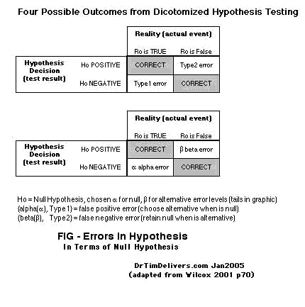
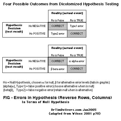
5. DICOTOMIZATION allows for 4 possible Test/Reality Situations, often shown as a 2x2 table (see A):
  
  Reality(R) is True .., Test(H) is Positive.. ( True... Positive, correct assertion)
  Reality(R) is False , Test(H) is Negative ( True.. Negative, correct assertion)
  Reality(R) is False , Test(H) is Positive.. ( False. Positive, type1 alpha error)
  Reality(R) is True .., Test(H) is Negative ( False Negative, type2 beta error)
  
  The actual Reality is not usually known, of course, which is the purpose of the test.
6. There are equivalent ways to display the same hypothesis relationship, so careful attention is demanded to how the items are actually arranged. For example, the 2x2 table [A] can be equivalently diagrammed by reversing Reality and Hypothesis, row with column [B].
  
  A(left), B(right)
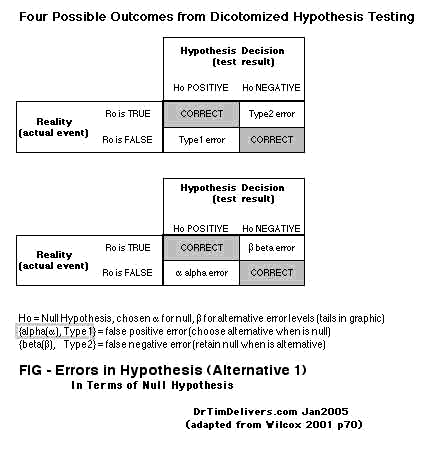
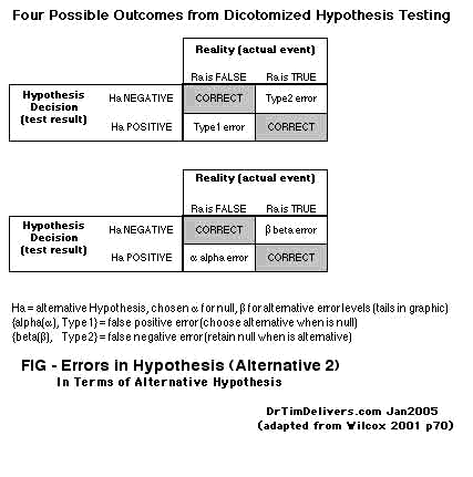
7. Still more ways diagram the findings in terms of the alternative hypothesis, rather than the null hypothesis:
  
  C(left),D(right)
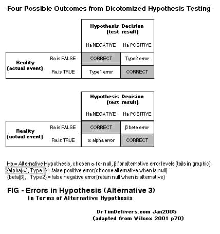
8. The R₀ & H₀ can be interchanged within a row or column as well, and all the previous can be recast (shown here only for A as E):
  
  E
9. It is important to discuss the two statistical errors in hypothesis testing (mucho confusing terminology)
  1. Type I error (see graphic of Hypothesis Testing below)
    1. alpha error, or "false finding" of difference from expected null (here alpha is used interchangeably for the cutoff level and probability in the null tail)
      1. false discard/rejection of null assumption, a false positive
      2. discard the null and accept the incorrect alternativehypotheses, or erroneously not retain the correct null hypothesis (hypothesis testing implies two conditions not just one)
      3. acceptance of alternative caused by chance when populations are actually the same, populations seem different but are not (a Type I error)
      4. distribution for the null determines the probability of an alpha error for given alpha cutoff
      5. choosing an alpha cutoff level for the null distrbution also fixes beta, the chance might erroneouslyreject the false alternative hypothesis (for a given alternative distribution and a given null mean. the alpha cutoff for the null is the beta cutoff for the alternative.)
    2. Significance (Null Probability related to alpha error)
      1. significance is how often correct when DO see effect
      2. determined by alpha cuttoff and null distribution
      3. true non-finding , correct retention/acceptance of null, true-negative of a difference from expected null
      4. significance is ( 1-alpha ) chance to correctly retain the true null hypothesis
      5. 95% null significance level (1-alpha) for a 5% Type I error level (alpha)
  2. Type II error (see graphic of Hypothesis Testing below)
    1. beta error, or "false ignoring" of a difference from expected null (here beta is used interchangeably for the cutoff level = X_c and probability in the alternative tail = function of X_c)
      1. false retention/acceptance of null, a false negative
      2. retain the null and reject the correct alternative hypothesis, or erroneously not discard the incorrect null hypothesis (hypothesis testing implies two conditions not just one)
      3. retention of null caused by chance when populations are actually different, populations seem the same but are not (a Type II error)
      4. distribution for the alternative determines the probability of an beta error for given cutoff
      5. choosing a beta cutoff level for the alternative distribution also fixes alpha, the chance might erroneouslyretain the false null hypothesis, (for a given null distribution and alternate mean. the beta cutoff for alternative is the alpha cutoff for the null.)
    2. Power (Alternative Probablity) related to beta error
      1. power is how often correct when DO NOT see effect
      2. determined by beta cutoff and alternative distribution
      3. true finding, correct rejection/non-retention of null, or true-positive of a difference from expected null
      4. power is (1-beta) chance to correctly accept the true alternative hypothesis
      5. 95% alternative power level (1-beta) for a 5% Type II error level (beta)
  3. [IMPORTANT ANOTE]
    1. Technically, the null and/or alternative can be negated, which recasts the expected null as false and alternative as true or whatever combination of the negations. These possibilities make craziness when following the logic of hypothesis testing. I have cast the issue here in the one way only for clarity and sanity. But perhaps research results would be much clearer if a standard approach was adopted and how one has to pay attention to this nitty gritty minutiae.
    2. If the observations are correlated, then the alpha and beta probablities are highly inaccurate (not discussed here). this violates the random selection assumption of summary statistics and is an important factor biasing results.
  4. Graphic Illustration of Hypothesis Testing Errors
    
    Shows the 6 parameters that must be limited to 2
    top graph error probabilities [alpha1, beta1]
    middle graph error probabilities [alpha1, beta2] same alpha/beta cutoff, different alternate mean, same alpha & different beta probablilities
    lower graph error probabilities [alpha2, beta2] different alpha/beta cutoff, same alternate mean, different alpha & beta probabilities
    
    [clic to enlarge]
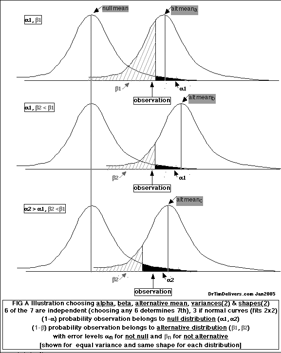
  5. Behavior of alpha significance, beta power
    1. error levels are always a compromise for given distributions and means - smaller alpha (fewer false positives) gives bigger beta (more false negatives), because they are not independent for fixed distributions
    2. smaller sample size for a normal distribution gives lower power = (1-beta)
    3. smaller standard deviation (variance of a distribution) gives higer power = (1-beta)
10. Z Test for significance with large sample size approximating a normal population distribution
  1. sample assumed from a normal curve
  2. standard deviation is known
  3. y_mean is the sample mean
  4. µ is the population mean
  5. Z = [ y_mean - µ ] / [ σ/SQRT(N) ] has a normal distribution
  6. can rule out chances a specific chosen value of the population mean µ, ie probablities are based on the mean of the alternative distribution
  7. Neyman, Pearson, Fisher developed (early 1900's)
  8. ok for large sample size N if population distribution approximates normal curve
11. One-Sample Student's T test used for significance with small samples and non-normal population distributions
  1. Laplace T distribution (1814, for large sample size n, p72-74)
    1. Laplace T = (y_mean- µ) / (S/ SQRT [n])
      1. y_mean is the sample mean
      2. µ is the population mean which is known
      3. problem if µ is not know
    2. Large sample size
      1. Laplace estimated the population standard deviation σ with the sample standard deviation S
      2. assumed the distribution of sample means has a normal distribution
        
        the difference between the population mean and the sample mean divided by the estimated standard error of the sample mean is normal, with mean=0 and variance=1
      3. central limit theorem for large sample size (large N) , T has a standard normal distribution with reasonably accurate probability coverage
    3. Small sample size
      1. Laplace T distribution is non-normal for small sample size N, even when sampled from a normal curve. using Z probablilities does not provide a good estimate of the probabilities for T distribution with small sample size (see Colton p128)
      2. when sampling from light-tailed curve, the probability curve for the sample means is approximately normal if the population distribution is not skewed (p74)
      3. if the distribution is skewed or heavy-tailed, large sample sizes are required
  2. Student's T Distribution (William Gossett 1908) (p74-76)
    1. T = (y_i -y_bar) / ([S/sqrt(n)])
      1. y_i= individual sample mean value
      2. y_bar = (1/n)(y₁ +y₂ +...+y_n ) = mean of all individual samples (Grand Mean of Sample Means)
      3. S² = [(1/(n-1)]*[(y₁ -y_bar ) ² + ... + (y_n -y_bar ) ² ] (Sample Variance for one sample)
      4. S/sqrt(n) = SE = SQRT (S²)
    2. note uses ybar for µ
    3. extension of Laplace T method, derived as approximation for the probability curve associated with T
    4. Ronald Fisher gave a more formal derivation
    5. probability depends on sample size
    6. assumes normality and random sampling
    7. although it is bell-shaped and centered about zero, T does not belong to the family of normal curves
      1. (T) has a standard deviation larger than 1, compared to normal (Z) distribution which has a mean of zero and standard deviation of 1
      2. T and Z are both symmetric (see Dawson 2001 Basic and Clinical Statistics p99)
      3. there are infinitely many bell curves that are not normal
    8. for large sample sizes, the probability curve associated with the T values becomes indistinguishable from the normal curve
      1. most computer programs always calculate T instead of Z even for large sample size
      2. T~Z for sample size of 5 or larger
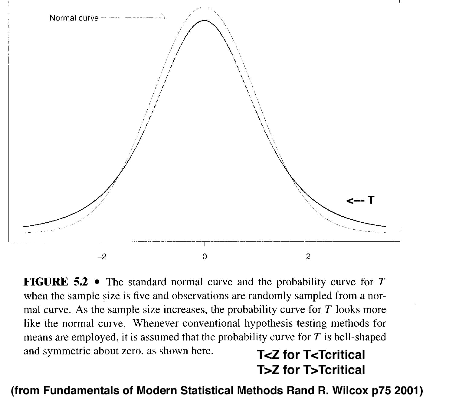
      3. for Tc<1.7, T < Z (T underestimates the probablity with 5 samples)
      4. for Tc>1.7, T > Z >(T overestimates the probability with 5 samples)
      5. [ANOTE]
        for a sample size of 5, calculating the Type I error (for alpha < .05 using Tc overestimates the area beyond Tc compared to the normal curve for Zc = Tc.
12. Practical Problems with Student's T (p77-81)
  1. serious inaccuracies can result for some nonnormal distributions
    1. in general, the sample mean and sample variance are dependent for T, that is the sample variance changes depending on the sample mean
    2. sample average for T is dependent on value and slopes around that value from the population distribution
    3. for normal curve mean and variance are independent
    4. Gossett's Student T can give exact confidence intervals and exact alpha Type I error for a normal population distribution, regardless of small sample size
    5. When sample from a lognormal distribution (example of skewed, light-tailed) actual probability curve for T differs
      1. plot of T distribution is skewed (longer tail) to smaller T in this case, and not symmetric about the mean compared to sampling from normal curve, sample size twenty (Fig 3.9, 5.5)
      2. mean of T distribution is shifted to smaller T (skewed to longer-tailed side as well) compared to the population distribution mean, because the population mean for the log-normal is shifted higher. that is
      3. T is biased to smaller values (although median is not shifted in the same manner).
    6. Alpha error can be inflated greater than the assumed level (underestimated). sometimes get a higher probability of rejecting when nothing is going on compared to when a difference actually exists
      1. Student T is then biased
      2. Expected Value E for the population of all individuals E[(Y-µ)²] = σ²
      3. Expected Value of the Sample Mean Y_bar is the population mean, or µ[E(Y_bar -µ) = 0]
      4. assumed that T is symmetric about zero (the expected value of T is zero, or the distribution of Y is symmetric about the mean) (p80)
        
        the Expected value of T must be zero if the mean and variance are independent, as under normality
        under non- normality, it does not necessarily follow that the mean of T is zero
      5. for skewed distribution, estimating the unknown variance with the sample variance in Student's T needs larger sample sizes to compensate to get accurate results for the mean and variance even when outliers are rare (light-tailed), increased to 200 for this example from 20.
      6. the actual probability of a Type I (alpha error) can be substantially higher than 0.05 at the 0.05 level
        
        occurs when the probability curve for T differs substantially from curve assuming normality
        [ISLT] this is a problem when comparing distributions that are skewed differently. Bootstrap techniques can estimate the probability curve for T to identify problem situations (Important newer techniques)
    7. Power can also be affected with Student's T (p82)
      1. the sample variance is more sensitive to outliers than the sample mean for Student's T Distribution
      2. even though the outliers inflate the sample mean, they can inflate the sample variance more
      3. this increases the confidence intervals for the mean of the distribution, and prevents finding an effect (rejecting the null) when compare different distributions, lowering power.
      4. [ISLT] this more of a problem for power when T distribution is skewed (distribution of means of samples from parent distribution), rather than when nonnormal and symmetric, or when the parent distribution is skewed
        
        evaluate symmetry of residuals for all sample means to check this
        implications of skewed vs heavy-tailed vs nonmonotonic (see ahead)
  2. Transforming the data can improve T approximation
    1. simple transformations sometimes correct serious problems with controlling Type I (alpha)
    2. typical strategy is to take logarithms of the observations and apply Student's T to the results
    3. simple transformations can fail to give satisfactory results in terms of achieving high power and relatively short confidence intervals (beta)
    4. other less obvious methods can be relatively more effective in these cases. sometimes have a higher probability of rejecting when nothing is going on, than when a difference actually exists
  3. Yuen's Method for difference of means (from Ch9)
    1. gives slightly better control of alpha error for large samples
      1. h is the number of observations left after trimming
      2. d₁ =(n₁-1)S_w1 ² / [h₁(h₁-1)]
      3. d₂ =(n₂-1)S_w2 ² / [h₂(h₂-1)]
      4. W = [(y_meant1 - y_meant2) - (µ_t1- µ_t2)] / [SQRT(d₁+d₂)]
    2. adding the Bootstrap Method to Yuen's Method may give better control of alpha error for small samples
  4. Welch's Test is another method that is generally more accurate than Student's T
13. Two-Sample Case for Means for significance with small samples (p82-83)
  
  Use Hypothesis of Equal Means to obtain the Confidence Interval for Difference of Means
  1. Difference between sample means estimates the difference between corresponding population means that samples are taken from
  2. LARGE Sample Size
    1. Weighted Two-Sample Difference = W
    2. assume large sample size (Laplace)
    3. assume random sampling
    4. no assumption about population variances
    5. n₁, n₂ are corresponding sample sizes
    6. Population Variance for weighted difference is
      1. Var(y_bar1 -y_bar2) = (σ₁)²/n₁ + (σ₂)²/n₂
    7. estimate this Population Variance with the Sample Variances (S₁,S₂)
      1. S² = (S₁)²/n₁+(S₂)²/n₂ SE = SQRT [S²] = SQRT [(S₁)²/n₁+(S₂)²/n₂]
    8. use the probabilities for the normal curve at 95%
      1. W = (y_bar1-y_bar2) / SE
        or
        W = (y_bar1-y_bar2) / SQRT[(S₁)²/n₁+(S₂)²/n₂]
      2. |W| > 1.96 = W_.95is the 95% confidence level to reject the hypothesis of equal means (from normal distribution)
      3. CI_.95 = (W_.95₎*SE = (+/-1.96)*SQRT[(S₁)²/n₁+(S₂)²/n₂]
    9. get a reasonably accurate confidence interval by the central limit theorem and good control over a Type 1 (alpha) error (better than Two-Sample T) if sample sizes are sufficiently large
    10. W gives somewhat better results for unequal population variances, although this is a serious problem, especially for power.
  3. SMALL Sample Size and Non-Normal distribution
    1. Two-Sample Difference T = T
    2. assume random sampling (Student/Gossett)
    3. assume equal Population Variances additionally
    4. n₁, n₂ are corresponding sample sizes
    5. For difference between sample means of two groups
      1. T = (y_bar1-y_bar2) / Sqrt[S_p²(1/n₁+1/n₂)]
        where the assumed common variance is
        S_p² = [(n₁-1)S₁²+(n₂-1)S₂²] / [n₁+n₂-2]
      2. the hypothesis of equal means is rejected if |T| > t (cutoff t is a function of degrees of freedom df and the confidence level, and obtained from tables based on Student's T distribution)
      3. CI_.95 = (t_.95(df)₎*SE = (+/-t_.95(df))*SQRT{[(n₁-1)S₁²+(n₂-1)S₂²] / [n₁+n₂-2]}
  4. W and T are equivalent for S₁ = S₂ (equal sample variances) or n₁ = n₂ (equal sample sizes)
14. Student Two-Sample T performs well under violations of assumptions (p84)
  1. Student Two-Sample T can substantially avoid inflation of Type I (alpha) errors, if the probability distributions
    1. are normal or have the same shape (ie, dont have differential skewness)
    2. have the same population variance
    3. have the same sample sizes
    4. then acceptable even for smaller samples
  2. Reliability of summary statistics for Two-SampleT distribution is affected by the shape and variance (of population or sample), and size (for samples). Unequal variances or differences in skewness can greatly affect the ability to detect true differences between means. (p 85, 86,122)
    
    1) same shape
    1. equal population variances
      1. alpha (Type 1) error should be fairly accurate
      2. normal or nonnormal-identical shape distributions
      3. same or different sample size
    2. unequal population variances
      1. same sample size with normal distributions
        
        sample size >8 , alpha (Type I) error is fairly accurate , no matter how unequal the variances
        sample size <8 , alpha (Type I) error can exceed 7.5% at the 5% level
      2. same sample size with nonnormal distributions, alpha (Type1) accuracy can be very poor
      3. different sample size with normal or nonnormal distributions, alpha (Type1) accuracy can be very poor
    2) different shape
    1. 1. alpha (type 1) accuracy can be very poor
      2. nonnormal and nonidentical distributions
      3. equal and unequal population variance / same and different samples of any size
15. Student T - Major Limitations (p86)
  1. Student's T test is not reliable with unequal population variances
    1. Student's T test can have very poor power (beta or false ignoring of effect, larger confidence intervals) for unequal population variances
      1. exacerbated with unequal population variances
      2. any method based on means can have low power
      3. expected value of one-sample T can differ from zero, and power can decrease as the effect gets greater for one-sample T test (the test is biased)
      4. [ANOTE] power decreases (T<1.7) but begins to go back up (T>1.7)
    2. Student's T test does not control the probability of a Type 1 error ( alpha or false finding ) for unequal population variances
      1. unequal distribution shapes, unequal variance, unequal sample size can cause problems in that order
      2. unequal variances with unequal sample sizes particularly can be a disaster for alpha error, even with equal sample sizes or normal distributions
      3. some argue that this is not a practical issue
    3. Difference between means may not represent the typical difference for two-sample T, because is the difference of inaccurate estimates of the population means
      1. W (Weighted T) helps avoid this compared to T for larger sample size
  2. Transforming the distributions can improve variance properties
    1. logarithm
    2. sample median (not a simple transformation in that some observations are given zero weight)
    3. Rasmussen (1989) reviewed this, found that low power due to outliers is still a problem
  3. When reject the null with Two-Sample Student T (find a difference), it is an indication that the probability distributions differ in some manner (distributions are not identical) (p87-89)
    1. if the population curves differ in some manner other than means, then the magnitude of any difference in the means becomes suspect (see limitations)
      1. population difference
        
        unequal means
        unequal variances
        difference in skew (shape)
        difference in other measure
      2. sampling difference
        
        unequal sample size
        non-randomization
    2. [ANOTE] a consideration is whether samples with equal sample variances would be likely to have unequal population variances, and thus create a problem using the Student T. If a study factor changes the population distribution (as evidenced by a variance difference), Student T would have problems for the difference of means.
  4. The difference between any two variables having identical skewness is a symmetric distribution. With a symmetric distribution, Type I significance errors are controlled reasonably well. But if the distributions differ in skewness, problems arise. Even under symmetry however, power might be a serious problem when comparing means.
  5. [ISLT] it is not so much that the population distributions themselves are skewed, but also factors which affect the derivatives of the distributions in different ways so that the difference curve is not symmetric (that is if skewing is not the same in both populations).
    1. normal curve has symmetric (linear) derivatives at any point along the curve
    2. light tailed curves would tend to have less problem (samples tend to be close to mean so symmetry is less of a problem)
    3. monotonic curves would tend to have less of this problem (exp, step, linear, exponential - samples tend to be symmetric about the mean)
    4. heavy tailed skewed curves have biased derivatives, so samples tend to favor one side of mean. also heavy tails would affect the variances even for symmetric curves.
    5. different population distributions would compare different biased means when determining differences (if the mean is biased the same way for in each group, when take the difference get accurate measure of difference of means)

The Bootstrap - Chapter 6*

One of the most robust techniques of all for means and variances are newer Bootstrap Techniques (a very important area not discussed here).

Trimmed Mean - Chapter 8 (p139-149)

"There has been an apparent errosion in the lines of communication between mathematical statisticians and applied researchers and these issues remain largely unknown. It is difficult even for statisticians to keep up. Quick explanations of modern methods are difficult. Some of the methods are not intuitive based on the standard training most applied researchers receive."
Issues about the sample mean (nonnormality)
1. nonnormality can result in very low power and poor assessment of effect size
  1. cannot find an estimator that is always optimal
  2. problem gets worse trying to measure the association between variables via least squares regression and Pearson's correlation
2. differences between probability curves other than the mean can affect conventional hypothesis testing between means
  1. population mean and population variance are not robust; they are sensitive to very small changes for any probability curve
  2. affects Student's T, and its generalization to multiple groups using the so-called ANOVA F-test.
  3. variance of mean is smaller than variance of median for normal curve, but variance of mean is larger than variance of median for mixed-normal distributions, even for a a very slight departure from normality
  4. George Box (1954) and colleagues
    1. sampling from normal distributions, unequal variances has no serious impact on the probability of a Type I (alpha) error
    2. if ratio of variances is less than 3, Type I (alpha) errors are generally controlled
      1. restrict ratio of the standard deviation of the largest group to the smallest at most sqrt(3)~2
      2. if this ratio gets larger, practical problems emerge
  5. Gene Glass (1972) and colleagues, and subsequent researchers
    1. indicate problems for unequal variances in the ability to control errors
    2. if groups differ in terms of both variances and skewness get unsatisfactory power properties (cant detect effects)
  6. H. Keselman (1998)
Summary of Factors affecting the probablities for the mean and variance
1. nonnormality and mixed normality (nonnormal contamination of normal population distribution)
  1. small departures from normality can inflate the population variance tremendously
2. heteroscedasticity, or changes in variance with predictor ( σ² ratio > 3 , σ ratio > 1.7)
  1. non-constant variance
  2. unless randomly affected rather than systematic
3. skew in population distribution
  1. asymmetry (very serious)
4. heavy tailed population distribution
  1. outliers dominate and can inflate the population variance tremendously
5. differences between probability curve distributions that are being compared
6. M-estimator and trimmed mean can improve these problems
M-estimators
1. for symmetric curves can give fairly accurate results
2. under even slight departures from symmetric curves, method breaks down especially for small sample size
3. also applies to two sample case
4. percentile bootstrap method performs better than percentile t method in combination with M-estimators for less than twenty observations
Percent Trimmed Mean [p143-149]
1. General Trimmed Mean
  1. advantages of 20% trimmed mean for the very common situation of of heavy-tailed probability curve
    1. sample variance is inflated for heavy-tailed compared to samples from a light-tailed distribution
    2. trimmed mean improves accuracy and precision for the mean
      1. tends to be substantially closer the the central value
    3. trimmed mean reduces the sample variance compared to the sample mean
      1. more likely to get high power and relatively short confidence intervals if use a trimmed mean rather than the sample mean
    4. symmetric vs skewed distributions does not affect this
  2. discards less accurate data that contaminates the population estimates
    1. for a normal curve or one with light tails , the sample mean is more accurate than the trimmed mean, but not substantially
    2. the middle values among a random sample of observations are much more likely to be close to the center of the normal curve.
    3. for the sample means, the extreme values hurt more than they help with even small departures from normality
    4. by trimming, in effect remove the heavy tails that bias the variance and thus the mean
    5. trimmed mean is not a weighted mean and not covered by the Gauss-Markov theorem, since it involves ordering the observations
      1. when remove extreme values the remaining observations are dependent
    6. breakdown point is 0.2 for the 20% trimmed mean
      1. the minimum proportion of outliers required to make the 20% trimmed mean arbitrarily large or small is 0.2 (20%)
      2. compare to the breakdown point of sample 1/n for the mean and 0.5 (50%) for the median
      3. arguments have been made that a sample breakdown point <0.1 is unwise
      4. so sample mean is awful relative to outliers
  3. for symmetric probability curves, the mean, median and trimmed mean of the population are all identical
    1. for a skewed one, all three generally differ
    2. when distributions are skewed, the median and 20% trimmed mean are argued to be better measures of what is typical (see Fig 8.3 p148)
  4. modern tools for characterizing the sensitivity of a parameter to small perturbations in a probability curve (since 1960)
    1. qualitative robustness
    2. infinitesimal robustness
    3. quantitative robustness (breakdown point of the sample mean for infinite sample size)
2. Gamma% Trimmed Mean
  1. Procedure
    1. determine N, the number of observations
    2. compute gamma*N (gamma= trim percentage)
    3. round down to the nearest integer = g
    4. remove the g smallest and g largest values (those with the largest deviations from the mean)
    5. average the n-2g values that remain
  2. Example: 20% Trimmed Mean (gamma=.2 or 20%)
    1. determine N, the number of observations
    2. compute 0.2*N
    3. round down to the nearest integer g
    4. remove the g smallest and g largest values (those with the largest deviations from the mean)
    5. average the (n-2g) values that remain

Variance of the Trimmed Mean - Chapter 9 (p159-178)

Variance of the sample trimmed mean refers to the variation among the infinitely many values from repeating a study infinitely many times
1. Computing the variance of the sample based on the data left after trimming the sample mean, and the standard error of the mean by dividing this by the number of samples (as do in computing the sample mean) is not satisfactory to obtain the trimmed variance
  1. usual variance of sample mean: if divide the sum of variables by n, the variance of the sum is divided by n
    1. Var(y_mean) = σ² / n
2. the trimmed mean observations are not independent (p162)
  1. the trimmed mean is an average of dependent variables and the sample mean method requires independence
  2. the variance of the sum of dependent variables is not equal to the sum of the individual variances, because the ordered variables are not independent
3. want to find the situations where the sample trimmed mean has a normal distribution
Estimating the sample trimmed mean, and variance of the sample trimmed mean (p162)
1. WINDSORIZE
  rewrite the trimmed mean as the average of the independent variables
2. COMPUTE Windsorized Sample Mean (Windsorized Mean) and the Sample Variance of the Windsorized mean (Windorized Sample Variance)
  1. put the observations in order
  2. trim gamma*n = g observations hi/lo (use Windsorized Variance)
    1. replace the trimmed values with the smallest of the non-trimmed values, so that the g smallest values are increased to the g+1th value not trimmed, and the g largest values likewise decreased (labled the W _n )
  3. subtract the Winsorized Mean from each of the Windsorized values, square each result, and then sum
  4. divide by n-1 (number of observations-1) as when computing the sample variance s ²
  5. Windsorized Sample Mean
    1. ybarw = (1/n)(W₁ +W₂ +...+W_n)
  6. Windsorized Sample Variance
    1. S_w² = [(1/(n-1)][(W₁ -ybar_w)² + ... + (W_n -ybar_w)²]
3. ADJUST the area under the curve for trimming to sum to probability of 1
  1. Estimated Variance of the Trimmed mean
    1. Var(ybar_T) = S_w² / (1-2 γ)² n
  2. 20%Trimmed mean Estimated Variance ( γ=.2, g=2, 1-2 γ=.6)
    1. Var(y_barT) = S_w² / (.36n) SD(y_bar ) = S_w / [.6 SQRT (n)]
4. Windsorized Variance for the trimmed mean is generally smaller than the simple sample variance, because it pulls in extreme values that inflate S²
  1. trimmed mean will be more accurate than the sample mean when it has a smaller variance
    1. for very small departure from normality, the variance of the trimmed mean can be substantially smaller
    2. the trimmed mean is relatively unaffected when sampling from the mixed normal curve
    3. true even when sampling from skewed distributions
  2. division by (1-2 γ)² could sometimes give the trimmed mean a larger variance than the sample mean, as when sampling from a normal parent curve, but typically any such improvement using the mean instead of trimmed mean is small
Standard Error of the Trimmed Mean (estimate of the Population trimmed mean)***
1. Small Sample Size (20% trimmed mean)
  1. Laplace Method approximation to the normal curve
  2. T_t = (y_bart - µ_t) / [S_w /.6sqrt(n)]
  3. CI = (+/-)t_crit(df)S_w / [.6sqrt(n)] = (+ / -)SE
  4. approximates the curve for Student T where df = n-2g-1 (degrees of freedom)
    1. for small sample sizes, the smaller the effect of non-normality up to 20% trimmed mean (less so as trim more)
    2. improves rapidly as sample size increases
  5. γ=0.2, g=2, n=12 case
    1. n-2g-1 = 12-4-1 = 7
    2. for 20% trim with 12 degrees of freedom at 95% confidence, T_crit = 2.365, ie., T _t >2.365 has probability <5%
    3. CI = (+ / -) 2.365S_w/[.6sqrt(n)]
2. 20% Trimmed Mean can be substantially more accurate than any method based on means, including the percentile bootstrap method
  1. indications are that can avoid alpha inaccuracies with sample sizes as small as 12 when combine the percentile bootstap method and the trimmed mean
    1. better control over alpha errors
    2. better power in a wide range of situations
    3. the problems of bias appear to be negligible (power decreasing as move away from the null hypothesis
    4. trimmed mean and sample mean are identical if sample from a symmetric population distribution
    5. if sample from skewed distribution, 20% trimmed mean is closer to the most likely values and provides a better reflection of the typical individual in the population
    6. confidence intervals for the trimmed mean is relatively insensitive to outliers (might be slightly altered when add the percentile bootstrap technique)
    7. does not eliminate all problems however, reduces them
Power using Trimmed Mean versus Simple Mean (p172)
1. confidence interval for the difference between trimmed means is considerably shorter than the confidence interval for the difference between sample means, because it is less affected by outliers
2. even small departures from normality can result in very low power (ability to detect an effect)
3. trimmed mean can reduce the problem of bias with a skewed distribution substantially
4. it is common to find situations where one fails to find a difference with means, but a difference is found with trimmed means.
5. it is rare for the reverse to happen, but it does happen
More issues about Student's T
1. how accurate the sample mean is for the population mean (estimates the population mean ), contrasted to how well the sample mean describes an individual in the population (estimates the population variance about the population mean)
2. probability curve for T may not be symmetric around zero because of non-normality and asymmetry
  1. 20% trimmed mean with a percentile bootstrap insures a more equi-tailed test, than when using a percentile T bootstrap with 20% trimmed mean
3. when comparing multiple groups, probability of an alpha error can drop well below the nominal level, and the power can be decreased. switching to a percentile bootstrap method with 20% trimmed mean can address this.
4. Percentile method using the 20% trimmed mean performs about as well as Student's T when making inferences about Means.
5. Percentile T method works better than percentile method in combination with the 20% trimmed mean as to shorter confidence intervals (Variances), and this improves for more than two groups
  1. theoretical results suggest that modifying the bootstrap method to Winsdorize before drawing bootstrap samples provides even shorter confidence intervals

Robust Regression - Chapter 11 (p206-228 selections)

Least Squares Regression
1. for probability of a Type I error (alpha error, seeing an effect that isnt there ) when testing the hypothesis of zero slope, least squares performs reasonably well.
  1. correlations between observations is a disaster for seeing an effect that isnt there (not discussed here)
2. if want to detect an association (small beta ) and describe that association (small CI ), least squares can fail miserably
  1. heterodscedasticity can result in relatively low power when testing the hypthesis that the slope is zero
  2. single unusual point can mask an important and interesting association
  3. nonnormality makes this worse, and the conventional methods for the slope can be highly inaccurate
3. when there is nonmormality or heteroscdedasticity, several additional methods compete well, and can be strikingly more accurate than Least Squares
  1. Theil-Sen Estimator
  2. Least Absolute Value Estimator
  3. Least Trimmed Squares
  4. Least Trimmed Absolute Value
  5. Least Median of Squares
  6. Adjusted M-estimator
  7. newer Empiric methods
  8. Deepest Regression Line (still being developed)
4. Using a regression estimator with a high breakdown point is no guarantee that disaster will be avoided with small sample sizes
  1. even among the robust regression estimators, the choice of method can make a practical difference
  2. a lower than max breakdown point may yield a more accurate estimate of the of the slope and intercept
  3. the example given (p 215) goes from a positive least squares estimate for slope (1.06, h=0 no trim), to a negative slope (-.62, h=.5n)
    1. using h=.8 (breakdown point =.2) gives a slope of 1.37
    2. for h=.75, gives a slope of .83
    3. Least median of squares estimate gives 1.36 (breakdown point of 0.5)
    4. Theil-Sen gives a slope of 1.01, which is more accurate than the least squares estimate
Least Trimmed Squares *** (p 212-215)
1. Procedure for Least Trimmed Squares :
  1. Ignore (trim) the largest residuals when calculating the variance used in the least square estimate
    1. order the residuals
    2. compute the variance based on the h=çn smallest residuals
      1. with ç=.5 (h=.5n), the breakdown point is .5, but the smallest value of ç that should be used is n/2 rounded down to the nearest integer plus 1
      2. ç > Int(n/2) + 1
    3. choose slope b1 and intercept b0 that minimizes this reduced variance for y=b0 +b1x line fit
  2. in effect by trimming them, removes the influence of the (n-h) largest residuals
  3. for h=.75n, ignores .25n in calculating the variance, so 25% of the points can be outliers without destroying the estimator
2. [ISLT] the problem of highly inaccurate estimate of the population mean by the sample mean arises when the trim process changes the sign of the parameter estimate (eg, slope estimate for Least Squares).
  1. may be general principle that regression estimators break down when they have sign change from the untrimmed estimate (third derivative of the curve changes at places of zero slope, consider population distribution versus sample distribution)
  2. this is a principle when linear fitting a sharply curved plot (non-monotonic compared to normal curve)
  3. need to identify points of zero slope and inflection so that estimates are contained in a place that is monotonic around the actual value, and not skip over a max or min that takes the estimate further away
  4. graphical or other diagnostic tools appear instrumental to identifying these situations - graph the data!
Regression Outliers and Leverage Points (p217)
1. Outliers
  1. regression outliers are points of the linear pattern that lie relatively far from the line around which most points are centered
  2. one way is to determine them is to use the least median squares regression line and compute the residuals using some criteria
2. Leverage Points
  1. unusually large or small X (predictor) values are called leverage points
  2. these points are heteroscedastic , with large residual (variance) for these large or small predictors
  3. good leverage point is one that has a large or small predictor value (X) , but is not a regression outlier (residual of Y from fit is small, doesnt affect slope or variance)
  4. bad leverage point is one that has a large Y residual for large or small predictor values (X) , and grossly affects the estimate of the slope
  5. the effect of outliers can affect the variance in a different way from the mean
    1. bad leverage points can lower the standard error while affecting the slope more despite the large (Y) residuals, since the larger the spread in predictor (X) values, the lower the standard error (SE) despite any leveraged outliers. but this can be more than offset by the inaccurate estimate of the slope.
    2. "rogue outliers" affect the slope less and the variance more by its leverage placement. y and x for the outliers are both inflated or deflated, so that Y/X keep close to the regression estimate although the variance is inflated.

Author Note about Sample Statistics

If the parent distributions don't really bunch around a central tendancy, are heavily skewed (bunched other than at the central tendancy) or are heavy-tailed, it is less accurate to use central tendancies to describe and compare them because the samples taken from those distributions can be biased.

The sample mean describes a distribution well (and regressions to find that mean) when the observations bunch up around a symmetric central tendancy without outliers. When there are outliers, Trimming helps the remaining observations to more accurately bunch for comparisons of means using the central tendancy. Differences of means for non-normal distributions are fairly reliable if the distributions have the same shape, but the probablities calculated from the Standard Error can be problematic.

"For example, the combination of the Percentile T Bootstrap and the 20 percent trimmed mean ... addresses all the problems with Student's T test, a result supported by both theory and simulation studies. The problem of bias appears to be negligible (power going down as the mean is further from the null hypothesis), we get vastly more accurate confidence intervals in situations where all methods based on means are deemed unsatisfactory, we get better control over Type I error probablilities, we get better power in a wider range of situations, and in the event sampling is from a normal curve, using means would offer only a slight advantage. When sampling from a probability curve that is symmetric, the population mean and trimmed mean are identical. But when sampling from a skewed curve [such as logheavy distribution], a 20 percent trimmed mean is closer to the most likely values and provides a better reflection of the typical individual under study." (p169)

The accuracy of probabilities and significance of differences depend on more than just the value of a central tendancy. The issue of comparing distributions that are skewed (same shapes or differing in shape) is a serious one, yet statistical techniques outlined here such as the trimmed mean, and newer bootstrap techniques (not discussed) offer powerful possibilities.

TDB

Top

back

goto www.DrTimDelivers.com

Counter

page views since July2012 (posted July 2005)